Calculations
Contents
Calculations
Surface Roughness Length
Equation from [UCAR, 2022]
\(z_{0}\) is the roughness length
\(z_{1}\) height of \(U_{1}\) (\(2 m\))
\(z_{2}\) height of \(U_{2}\) (\(10 m\))
\(k\) is the Von Karmon constant (\(0.4\))
\(u*\) is friction velocity (measured, in flux dataset)
\(U_{1}\) wind speed at \(z_{1}\) (measued, in meteorology dataset)
\(U_{2}\) wind speed at \(z_{2}\) (measued, in meteorology dataset)
import matplotlib.pyplot as plt

import pandas as pd
import xarray as xr
import numpy as np

import json
import time
import datetime
import glob

import warnings
warnings.filterwarnings('ignore')

plt.style.use('default')
# Wind speed at 2 m
u1 = xr.open_dataset('/Users/smurphy/all_datasets/nice_published_datasets/N-ICE_metData_v2.nc',
                     decode_times = False)['wind_speed_2m'].mean().values

# Wind speed at 10 m
u2 = xr.open_dataset('/Users/smurphy/all_datasets/nice_published_datasets/N-ICE_metData_v2.nc',
                     decode_times = False)['wind_speed_10m'].mean().values

# Friction velocity
ustar = xr.open_dataset('/Users/smurphy/all_datasets/nice_published_datasets/N-ICE_sebData_v1.nc',
                        decode_times = False)['friction_velocity'].mean().values

# Heights
z1 = 2 # m
z2 = 10 # m

# Von Karmon Constant
k  = 0.4

# Calculation
term1 = (z2 - z1)
term2 = np.exp((k * u2) / ustar)
term3 = np.exp((k * u1) / ustar)
z = term1 / (term2 - term3)

print('Surface Roughness Length (m):')
z
Surface Roughness Length (m):
0.0012378941216551337
I calculated the above surface roughness length using \(z_{2} = 4m\) and \(z_{2} = 10m\) (and modified \(U_{2}\) accordingly) and found both heights gave similar results.
We have roughness length from EddyPro, how does this match up to my calculated roughness length?
EddyPro calculates roughness length using the canopy height: $\(z_{0} = 0.15 * canopy\ height\)\( Canopy height is defined as \)0$ in our EddyPro runs [LI-COR, 2021].
roughness_length = pd.DataFrame(columns = ['Jan','Feb','Mar','Apr','May','Jun'])

for mon in ['Jan','Feb','Mar','Apr','May','Jun']:
    path = glob.glob('/Volumes/509_data/EddyPro/Output/EddyPro_Runs/FDCorrected_Output/20hz/' + mon + '/eddypro_sonic_essentials_*')
    mean_rl = pd.read_csv(path[0],
                          index_col = 0)['roughness_length'].mean()
    roughness_length[mon] = [mean_rl]

roughness_length = roughness_length.T
roughness_length.columns = ['z']
print(roughness_length)
---------------------------------------------------------------------------
IndexError                                Traceback (most recent call last)
/var/folders/21/bhksj_cn7zz43y8x0m4gsh0h0000gn/T/ipykernel_54799/2827172348.py in <module>
      3 for mon in ['Jan','Feb','Mar','Apr','May','Jun']:
      4     path = glob.glob('/Volumes/509_data/EddyPro/Output/EddyPro_Runs/FDCorrected_Output/20hz/' + mon + '/eddypro_sonic_essentials_*')
----> 5     mean_rl = pd.read_csv(path[0],
      6                           index_col = 0)['roughness_length'].mean()
      7     roughness_length[mon] = [mean_rl]

IndexError: list index out of range
So, I believe it’s safe to say we can be confident in my roughness length calculations.
Surface Heat Capacity
Sea Ice Thermodynamics [UCAR, 2017] equation 12
\(c(T,S)\) is the heat capacity, \(\frac{J}{kg K}\)
\(c_{0}\) is the heat capacity of fresh ice, \(2054 \frac{J}{kg K}\)
\(L_{i}\) is the latent heat of fusion, \(3.340 * 10^{5} \frac{J}{kg}\)
\(S\) is the salinity (we have salinity from the ice measurements), \(ppt\)
\(T\) is temperature (we have ice surface temperature from the ice measurements), \(K\)
\(\mu\) is the ocean freezing temperature constant and is directly related to salinity, \(0.054 \frac{^{\circ} C}{ppt}\)
# Importing variables from the Sea Ice Physics dataset
# Sea ice salinity and surface temperature to be used in the surface heat capacity calculations
# Density to be used in this calculation for the thermal inertia constant

with open('/Users/smurphy/all_datasets/nice_published_datasets/n-ice2015-ice-core-physics.json') as f:
    data = json.load(f)
keys, vals = data.items()

density_df = pd.DataFrame()
for i in np.arange(0,len(vals[1]),1):
    if 'density' in vals[1][i].keys():
        mean_level = (np.array(vals[1][i]['sample_top_cm'], dtype=np.float)[~np.isnan(np.array(vals[1][i]['density'], dtype=np.float))] - np.array(vals[1][i]['sample_bottom_cm'], dtype=np.float)[~np.isnan(np.array(vals[1][i]['density'], dtype=np.float))])/2
        den_vals = np.array(vals[1][i]['density'], dtype = np.float)[~np.isnan(np.array(vals[1][i]['density'], dtype = np.float))]
        density_temp_df = pd.DataFrame(data = den_vals.reshape(1, len(den_vals)),
                                       columns = mean_level,
                                       index = [datetime.datetime.strptime(vals[1][i]['properties']['time'],"%Y-%m-%dT%H:%M:%SZ")])
        density_df = pd.concat([density_df, density_temp_df], axis=1)

salinity_df = pd.DataFrame()
for i in np.arange(0,len(vals[1]),1):
    if 'sea_ice_salinity' in vals[1][i].keys():
        den_vals = np.mean(np.array(vals[1][i]['sea_ice_salinity'], dtype = np.float)[~np.isnan(np.array(vals[1][i]['sea_ice_salinity'], dtype = np.float))])
        salinity_temp_df = pd.DataFrame(data = [den_vals],
                                       index = [datetime.datetime.strptime(vals[1][i]['properties']['time'],"%Y-%m-%dT%H:%M:%SZ")])
        salinity_df = pd.concat([salinity_df, salinity_temp_df], axis=1)

surft_df = pd.DataFrame()
for i in np.arange(0,len(vals[1]),1):
    if 'surface_temperature' in vals[1][i]['properties'].keys():
        den_vals = np.array(vals[1][i]['properties']['surface_temperature'], dtype = np.float)[~np.isnan(np.array(vals[1][i]['properties']['surface_temperature'], dtype = np.float))]
        surftemp_temp_df = pd.DataFrame(data = [den_vals],
                                       index = [datetime.datetime.strptime(vals[1][i]['properties']['time'],"%Y-%m-%dT%H:%M:%SZ")])
        surft_df = pd.concat([surft_df, surftemp_temp_df], axis=1)
What value of temperature should I use?
f1 = surft_df['2015-01-01':'2015-02-21']
f2 = surft_df['2015-02-23':'2015-03-21']
f3 = surft_df['2015-04-18':'2015-06-05']
f4 = surft_df['2015-06-07':'2015-06-21']

wint = surft_df['2015-01-01':'2015-04-01']
summ = surft_df['2015-04-07':'2015-06-21']

plt.figure(figsize = (10,5))
plt.plot(surft_df.mean(axis = 1), 'o', alpha = 0.75)

plt.axhline(surft_df.mean(axis = 1).mean(), linestyle = ':', linewidth = 2)

plt.hlines(f1.mean(axis = 1).mean(), xmin = '2015-01-01', xmax = '2015-02-21', linestyle = '--', color = 'g')
plt.hlines(f2.mean(axis = 1).mean(), xmin = '2015-02-23', xmax = '2015-03-21', linestyle = '--', color = 'r')
plt.hlines(f3.mean(axis = 1).mean(), xmin = '2015-04-18', xmax = '2015-06-05', linestyle = '--', color = 'purple')
plt.hlines(f4.mean(axis = 1).mean(), xmin = '2015-06-07', xmax = '2015-06-21', linestyle = '--', color = 'blue')

plt.hlines(wint.mean(axis = 1).mean(), xmin = '2015-01-01', xmax = '2015-04-01', linestyle = '--', color = 'pink')
plt.hlines(summ.mean(axis = 1).mean(), xmin = '2015-04-07', xmax = '2015-06-21', linestyle = '--', color = 'cyan')

plt.ylabel('Ice Surface Temperature $(^{\circ}c)$')
plt.title('Ice Surface Temperature')
plt.grid()
plt.legend(['Measurements', 'Experiment Mean: ' + str(np.round(surft_df.mean(axis = 1).mean(),2)) + ' c',
            'Floe 1 Mean:          ' + str(np.round(f1.mean(axis = 1).mean(),2)) + ' c',
            'Floe 2 Mean:          ' + str(np.round(f2.mean(axis = 1).mean(),2)) + ' c',
            'Floe 3 Mean:            ' + str(np.round(f3.mean(axis = 1).mean(),2)) + ' c',
            'Floe 4 Mean:             ' + str(np.round(f4.mean(axis = 1).mean(),2)) + ' c',
            'Winter Mean:          ' + str(np.round(wint.mean(axis = 1).mean(),2)) + ' c',
            'Summer Mean:         ' + str(np.round(summ.mean(axis = 1).mean(),2)) + ' c']);
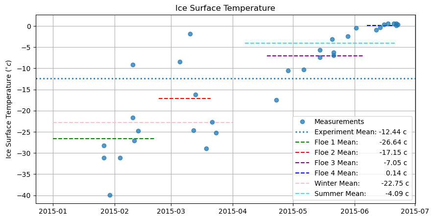
print('Ice surface temperature (c)')
np.round(surft_df.mean(axis = 1).mean(),2)
Ice surface temperature (c)
-12.44
print('Winter surface temperature')
np.round(surft_df['2015-01-01':'2015-04-01'].mean(axis = 1).mean(),2)
Winter surface temperature
-22.75
print('Summer surface temperature')
np.round(surft_df['2015-04-07':'2015-06-21'].mean(axis = 1).mean(),2)
Summer surface temperature
-4.09
How does this temperature compare to the surface temperature that Von calculated?
atmospheric_surface_temperature = pd.read_excel('/Users/smurphy/Documents/PhD/datasets/nice_data/Ts.xlsx', index_col = 0, parse_dates = True)
f1 = (atmospheric_surface_temperature - 273.15)['2015-01-01':'2015-02-21']
f2 = (atmospheric_surface_temperature - 273.15)['2015-02-23':'2015-03-21']
f3 = (atmospheric_surface_temperature - 273.15)['2015-04-18':'2015-06-05']
f4 = (atmospheric_surface_temperature - 273.15)['2015-06-07':'2015-06-21']

wint = (atmospheric_surface_temperature - 273.15)['2015-01-01':'2015-04-01']
summ = (atmospheric_surface_temperature - 273.15)['2015-04-07':'2015-06-21']

plt.figure(figsize = (10,5))
plt.plot(surft_df.mean(axis = 1), 'o', alpha = 0.75)
plt.plot(atmospheric_surface_temperature - 273.15, alpha=0.5)

plt.axhline(surft_df.mean(axis = 1).mean(), linestyle = ':', linewidth = 2)

plt.hlines(f1.mean(axis = 1).mean(), xmin = '2015-01-01', xmax = '2015-02-21', linestyle = '--', color = 'g')
plt.hlines(f2.mean(axis = 1).mean(), xmin = '2015-02-23', xmax = '2015-03-21', linestyle = '--', color = 'r')
plt.hlines(f3.mean(axis = 1).mean(), xmin = '2015-04-18', xmax = '2015-06-05', linestyle = '--', color = 'purple')
plt.hlines(f4.mean(axis = 1).mean(), xmin = '2015-06-07', xmax = '2015-06-21', linestyle = '--', color = 'blue')

plt.hlines(wint.mean(axis = 1).mean(), xmin = '2015-01-01', xmax = '2015-04-01', linestyle = '--', color = 'pink')
plt.hlines(summ.mean(axis = 1).mean(), xmin = '2015-04-07', xmax = '2015-06-21', linestyle = '--', color = 'cyan')


plt.ylabel('Ice Surface Temperature $(^{\circ}c)$')
plt.title('Ice Surface Temperature')
plt.grid()
plt.legend(['Ice Measurements',
            'Surface Temperture from\nAtmospheric Measurements',
            'Experiment Mean: ' + str(np.round((atmospheric_surface_temperature - 273.15).mean()[0],2)) + ' c',
            'Floe 1 Mean:          ' + str(np.round(f1.mean(axis = 1).mean(),2)) + ' c',
            'Floe 2 Mean:          ' + str(np.round(f2.mean(axis = 1).mean(),2)) + ' c',
            'Floe 3 Mean:            ' + str(np.round(f3.mean(axis = 1).mean(),2)) + ' c',
            'Floe 4 Mean:             ' + str(np.round(f4.mean(axis = 1).mean(),2)) + ' c',
            'Winter Mean:          ' + str(np.round(wint.mean(axis = 1).mean(),2)) + ' c',
            'Summer Mean:         ' + str(np.round(summ.mean(axis = 1).mean(),2)) + ' c',]);
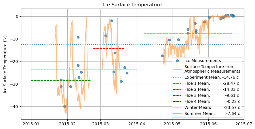
The dashed line means in this figure represent means of the orange line
print('Winter surface temperature')
np.round((atmospheric_surface_temperature - 273.15)['2015-01-01':'2015-04-01'].mean(axis = 1).mean(),2)
Winter surface temperature
-23.57
print('Summer surface temperature')
np.round((atmospheric_surface_temperature - 273.15)['2015-04-07':'2015-06-21'].mean(axis = 1).mean(),2)
Summer surface temperature
-7.64
This doesn’t change much, but I’ll use our valaues of surface temperature for the calculations.
What value of salinity should I use?
f1 = salinity_df['2015-01-01':'2015-02-21']
f2 = salinity_df['2015-02-23':'2015-03-21']
f3 = salinity_df['2015-04-18':'2015-06-05']
f4 = salinity_df['2015-06-07':'2015-06-21']

wint = salinity_df['2015-01-01':'2015-04-01']
summ = salinity_df['2015-04-07':'2015-06-21']

plt.figure(figsize = (10,5))
plt.plot(salinity_df.mean(axis = 1), 'o')
plt.axhline(salinity_df.mean(axis = 1).mean(), linestyle = ':', linewidth = 2)

plt.hlines(f1.mean(axis = 1).mean(), xmin = '2015-01-01', xmax = '2015-02-21', linestyle = '--', color = 'g')
plt.hlines(f2.mean(axis = 1).mean(), xmin = '2015-02-23', xmax = '2015-03-21', linestyle = '--', color = 'r')
plt.hlines(f3.mean(axis = 1).mean(), xmin = '2015-04-18', xmax = '2015-06-05', linestyle = '--', color = 'purple')
plt.hlines(f4.mean(axis = 1).mean(), xmin = '2015-06-07', xmax = '2015-06-21', linestyle = '--', color = 'blue')

plt.hlines(wint.mean(axis = 1).mean(), xmin = '2015-01-01', xmax = '2015-04-01', linestyle = '--', color = 'pink')
plt.hlines(summ.mean(axis = 1).mean(), xmin = '2015-04-07', xmax = '2015-06-21', linestyle = '--', color = 'cyan')

plt.ylabel('Mean Ice Core Salinity $(g/kg)$')
plt.title('Ice Core Salinity')
plt.grid()

plt.legend(['Measurements', 'Experiment Mean:    ' + str(np.round(salinity_df.mean(axis = 1).mean(),2)) + ' g/kg',
            'Floe 1 Mean:               ' + str(np.round(f1.mean(axis = 1).mean(),2)),
            'Floe 2 Mean:             ' + str(np.round(f2.mean(axis = 1).mean(),2)) + ' g/kg',
            'Floe 3 Mean:             ' + str(np.round(f3.mean(axis = 1).mean(),2)) + ' g/kg',
            'Floe 4 Mean:             ' + str(np.round(f4.mean(axis = 1).mean(),2)) + ' g/kg',
            'Winter Mean:            ' + str(np.round(wint.mean(axis = 1).mean(),2)) + ' g/kg',
            'Summer Mean:         ' + str(np.round(summ.mean(axis = 1).mean(),2)) + ' g/kg'], loc = 'upper left');
/Users/smurphy/opt/anaconda3/lib/python3.8/site-packages/numpy/core/_asarray.py:83: UserWarning: Warning: converting a masked element to nan.
  return array(a, dtype, copy=False, order=order)
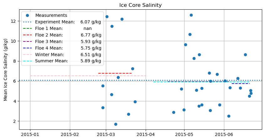
print('Mean Ice Core Salinity: (g/kg)')
np.round(salinity_df.mean(axis = 1).mean(),2)
Mean Ice Core Salinity: (g/kg)
6.07
Calculating
Before we calculate this, let’s remind ourselves of the equation:
\(c(T,S)\) is the heat capacity, \(\frac{J}{kg K}\)
\(c_{0}\) is the heat capacity of fresh ice, \(2054 \frac{J}{kg K}\)
\(L_{i}\) is the latent heat of fusion, \(3.340 * 10^{5} \frac{J}{kg}\)
\(S\) is the salinity (we have salinity from the ice measurements), \(ppt\) (parts per thousand)
\(T\) is temperature (we have ice surface temperature from the ice measurements), \(K\)
\(\mu\) is the ocean freezing temperature constant and is directly related to salinity, \(0.054 \frac{^{\circ} C}{ppt}\)
#                                                                                      ** Desired units for each value
# Salinity
s = np.round(salinity_df.mean(axis = 1).mean(),2) # g / kg = ppt                       ** ppt (parts per THOUSAND)

# Ocean freezing temperature constant
mu = 0.054 # c / ppt                                                                   ** K

# Heat capacity of fresh ice
c0 = 2054 # J / (kg K)                                                                 ** J/(kg K)

# Ice surface temperature
t = np.round(atmospheric_surface_temperature.mean(),2) # K                             ** K

# Ice surface temperature - Summer
t_s = np.round(atmospheric_surface_temperature['2015-04-07':'2015-06-21'].mean(),2) #  ** K

# Ice surface temperature - Winter
t_w = np.round(atmospheric_surface_temperature['2015-01-01':'2015-04-01'].mean(),2) #  ** K

# Latent heat of fusion
li = 3.340 * 10 ** 5 # J / kg                                                          ** J/kg

# Calculating
c = c0 + ((li * mu * s) / (t**2))       # using mean temperature of entire experiment
c_w = c0 + ((li * mu * s) / (t_w**2))   # using mean winter temperature
c_s = c0 + ((li * mu * s) / (t_s**2))   # using mean summer/spring temperature

print('Surface Heat Capacity (J/(kg k)):')
print("{:e}".format(c[0]))
Surface Heat Capacity (J/(kg k)):
2.055640e+03
print('Winter Surface Heat Capacity (J/(kg k)):')
print("{:e}".format(c_w[0]))
Winter Surface Heat Capacity (J/(kg k)):
2.055758e+03
print('Summer Surface Heat Capacity (J/(kg k)):')
print("{:e}".format(c_s[0]))
Summer Surface Heat Capacity (J/(kg k)):
2.055553e+03
Can we trust this calculation?
First, let’s plot \(\frac{L_{i}\mu S}{T^{2}}\) since this is the correction term.
Units?
\(\frac{\frac{J}{kg} \frac{K}{ppt} ppt}{K^{2}} = \frac{\frac{J}{kg}}{K} \)
plt.figure(figsize = (10,5))

f1 = ((li * mu * s) / ((surft_df.mean(axis = 1)+273.15)**2))['2015-01-01':'2015-02-21']
f2 = ((li * mu * s) / ((surft_df.mean(axis = 1)+273.15)**2))['2015-02-23':'2015-03-21']
f3 = ((li * mu * s) / ((surft_df.mean(axis = 1)+273.15)**2))['2015-04-18':'2015-06-05']
f4 = ((li * mu * s) / ((surft_df.mean(axis = 1)+273.15)**2))['2015-06-07':'2015-06-21']

wint = ((li * mu * s) / ((surft_df.mean(axis = 1)+273.15)**2))['2015-01-01':'2015-04-01']
summ = ((li * mu * s) / ((surft_df.mean(axis = 1)+273.15)**2))['2015-04-07':'2015-06-21']

plt.plot(((li * mu * s) / ((surft_df.mean(axis = 1)+273.15)**2)), 'o')
plt.axhline(((li * mu * s) / ((surft_df.mean(axis = 1)+273.15)**2)).mean(), linestyle = ':', linewidth = 2)

plt.hlines(f1.mean(), xmin = '2015-01-01', xmax = '2015-02-21', linestyle = '--', color = 'g')
plt.hlines(f2.mean(), xmin = '2015-02-23', xmax = '2015-03-21', linestyle = '--', color = 'r')
plt.hlines(f3.mean(), xmin = '2015-04-18', xmax = '2015-06-05', linestyle = '--', color = 'purple')
plt.hlines(f4.mean(), xmin = '2015-06-07', xmax = '2015-06-21', linestyle = '--', color = 'blue')

plt.hlines(wint.mean(), xmin = '2015-01-01', xmax = '2015-04-01', linestyle = '--', color = 'pink')
plt.hlines(summ.mean(), xmin = '2015-04-07', xmax = '2015-06-21', linestyle = '--', color = 'cyan')

plt.grid()
plt.title('Correction Term in Surface Heat Capacity')
plt.ylabel('Correction Term $(J/(kg \ K))$')
plt.xlabel('Date');

plt.legend(['Correction Term',
            'Mean Correction: ' + "{:.2}".format(((li * mu * s) / ((surft_df.mean(axis = 1)+273.15)**2)).mean()) + ' J/(kg K)',
            'Floe 1 Mean:        ' + "{:.2}".format(f1.mean()) + ' J/(kg K)',
            'Floe 2 Mean:        ' + "{:.2}".format(f2.mean()) + ' J/(kg K)',
            'Floe 3 Mean:        ' + "{:.2}".format(f3.mean()) + ' J/(kg K)',
            'Floe 4 Mean:        ' + "{:.2}".format(f4.mean()) + ' J/(kg K)',
            'Winter Mean:       ' + "{:.2}".format(wint.mean()) + ' J/(kg K)',
            'Summer Mean:    ' + "{:.2}".format(summ.mean()) + ' J/(kg K)'],
           loc = 'upper right');
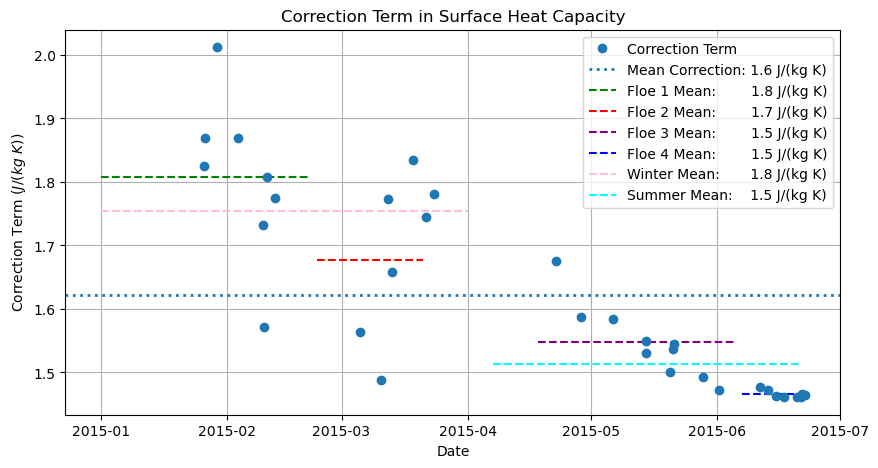
The value of \(\mu\) is the determining factor for how large this value is
plt.figure(figsize = (10,5))

f1 = c0 + ((li * mu * s) / ((surft_df.mean(axis = 1)+273.15)**2))['2015-01-01':'2015-02-21']
f2 = c0 + ((li * mu * s) / ((surft_df.mean(axis = 1)+273.15)**2))['2015-02-23':'2015-03-21']
f3 = c0 + ((li * mu * s) / ((surft_df.mean(axis = 1)+273.15)**2))['2015-04-18':'2015-06-05']
f4 = c0 + ((li * mu * s) / ((surft_df.mean(axis = 1)+273.15)**2))['2015-06-07':'2015-06-21']

wint = c0 + ((li * mu * s) / ((surft_df.mean(axis = 1)+273.15)**2))['2015-01-01':'2015-04-01']
summ = c0 + ((li * mu * s) / ((surft_df.mean(axis = 1)+273.15)**2))['2015-04-07':'2015-06-21']

plt.plot(c0 + ((li * mu * s) / ((surft_df.mean(axis = 1)+273.15)**2)), 'o')
plt.axhline(c0 + ((li * mu * s) / ((surft_df.mean(axis = 1)+273.15)**2)).mean(), linestyle = ':', linewidth = 2)

plt.hlines(f1.mean(), xmin = '2015-01-01', xmax = '2015-02-21', linestyle = '--', color = 'g')
plt.hlines(f2.mean(), xmin = '2015-02-23', xmax = '2015-03-21', linestyle = '--', color = 'r')
plt.hlines(f3.mean(), xmin = '2015-04-18', xmax = '2015-06-05', linestyle = '--', color = 'purple')
plt.hlines(f4.mean(), xmin = '2015-06-07', xmax = '2015-06-21', linestyle = '--', color = 'blue')

plt.hlines(wint.mean(), xmin = '2015-01-01', xmax = '2015-04-01', linestyle = '--', color = 'pink')
plt.hlines(summ.mean(), xmin = '2015-04-07', xmax = '2015-06-21', linestyle = '--', color = 'cyan')

plt.grid()
plt.title('Surface Heat Capacity')
plt.ylabel('Heat Capacity $(J/(kg \ K))$')
plt.xlabel('Date');

plt.legend(['Surface Heat Capacity',
            'Mean Heat Capacity: ' + "{:.2}".format(c0 + ((li * mu * s) / ((surft_df.mean(axis = 1)+273.15)**2)).mean()) + ' J/(kg K)',
            'Floe 1 Mean:              ' + "{:.2}".format(f1.mean()) + ' J/(kg K)',
            'Floe 2 Mean:              ' + "{:.2}".format(f2.mean()) + ' J/(kg K)',
            'Floe 3 Mean:              ' + "{:.2}".format(f3.mean()) + ' J/(kg K)',
            'Floe 4 Mean:              ' + "{:.2}".format(f4.mean()) + ' J/(kg K)',
            'Winter Mean:             ' + "{:.2}".format(wint.mean()) + ' J/(kg K)',
            'Summer Mean:          ' + "{:.2}".format(summ.mean()) + ' J/(kg K)'],
           loc = 'upper right');
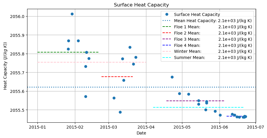
The correction term is clearly dominating the surface heat capacity. To get it into the correct units, we need to multiply this by the ice density.
f1 = density_df['2015-01-01':'2015-02-21']
f2 = density_df['2015-02-23':'2015-03-21']
f3 = density_df['2015-04-18':'2015-06-05']
f4 = density_df['2015-06-07':'2015-06-21']

wint = density_df['2015-01-01':'2015-04-01']
summ = density_df['2015-04-07':'2015-06-21']

plt.figure(figsize = (10,5))
plt.plot(density_df.mean(axis = 1), 'o', alpha = 0.75)

plt.axhline(density_df.mean(axis = 1).mean(), linestyle = ':', linewidth = 2)

plt.hlines(f1.mean(axis = 1).mean(), xmin = '2015-01-01', xmax = '2015-02-21', linestyle = '--', color = 'g')
plt.hlines(f2.mean(axis = 1).mean(), xmin = '2015-02-23', xmax = '2015-03-21', linestyle = '--', color = 'r')
plt.hlines(f3.mean(axis = 1).mean(), xmin = '2015-04-18', xmax = '2015-06-05', linestyle = '--', color = 'purple')
plt.hlines(f4.mean(axis = 1).mean(), xmin = '2015-06-07', xmax = '2015-06-21', linestyle = '--', color = 'blue')

plt.hlines(wint.mean(axis = 1).mean(), xmin = '2015-01-01', xmax = '2015-04-01', linestyle = '--', color = 'pink')
plt.hlines(summ.mean(axis = 1).mean(), xmin = '2015-04-07', xmax = '2015-06-21', linestyle = '--', color = 'cyan')

plt.ylabel('Density $(kg/m^{3})$')
plt.title('Ice Density')
plt.ylim(800, 950)
plt.grid()
plt.legend(['Measurements', 'Experiment Mean: ' + str(np.round(density_df.mean(axis = 1).mean(),2)) + ' kg/m3',
            'Floe 1 Mean:          ' + str(np.round(f1.mean(axis = 1).mean(),2)) + ' kg/m3',
            'Floe 2 Mean:          ' + str(np.round(f2.mean(axis = 1).mean(),2)) + ' kg/m3',
            'Floe 3 Mean:          ' + str(np.round(f3.mean(axis = 1).mean(),2)) + ' kg/m3',
            'Floe 4 Mean:             ' + str(np.round(f4.mean(axis = 1).mean(),2)),
            'Winter Mean:         ' + str(np.round(wint.mean(axis = 1).mean(),2)) + ' kg/m3',
            'Summer Mean:      ' + str(np.round(summ.mean(axis = 1).mean(),2)) + ' kg/m3'], loc = 'lower center');
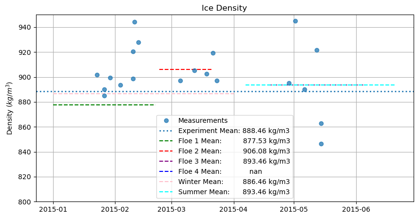
print('Ice density (kg/m3)')
np.round(density_df.mean(axis = 1).mean(),2)
Ice density (kg/m3)
888.46
c = c * density_df.mean(axis = 1).mean()   # J/(kg K) * kg/m3 = J/(m3 K)
c_w = c_w * density_df.mean(axis = 1).mean()   # J/(kg K) * kg/m3 = J/(m3 K)
c_s = c_s * density_df.mean(axis = 1).mean()   # J/(kg K) * kg/m3 = J/(m3 K)
print('Surface Heat Capacity (J/(m3 K))')
print("{:e}".format(c[0]))
Surface Heat Capacity (J/(m3 K))
1.826350e+06
print('Winter - Surface Heat Capacity (J/(m3 K))')
print("{:e}".format(c_w[0]))
Winter - Surface Heat Capacity (J/(m3 K))
1.826455e+06
print('Summer - Surface Heat Capacity (J/(m3 K))')
print("{:e}".format(c_s[0]))
Summer - Surface Heat Capacity (J/(m3 K))
1.826273e+06
Albedo
What is the exact albedo throughout the experiment? We used a value of .8 for the simulations, but what is the actual value for each season? We have these measurements from N-ICE.
# Importing and formatting the albedo dataset
albedo_dataset = xr.open_dataset('/Users/smurphy/Documents/PhD/datasets/nice_data/N-ICE_albedoData_v1.nc')
albedo_dataframe = pd.DataFrame(columns = ['albedo', 'month', 'day'])
albedo_dataframe['albedo'] = albedo_dataset.surface_albedo_mean.values
albedo_dataframe['month'] = albedo_dataset.month.values
albedo_dataframe['day'] = albedo_dataset.day.values
albedo_dataframe.index = ['2015-0' + x + '-' for x in albedo_dataframe.month.values.astype(int).astype(str)] + albedo_dataframe['day'].dt.days.astype(str)
albedo_dataframe.index = pd.to_datetime(albedo_dataframe.index)
albedo_dataframe = albedo_dataframe['albedo']
f1 = albedo_dataframe['2015-01-01':'2015-02-21']
f2 = albedo_dataframe['2015-02-23':'2015-03-21']
f3 = albedo_dataframe['2015-04-18':'2015-06-05']
f4 = albedo_dataframe['2015-06-07':'2015-06-21']

wint = albedo_dataframe['2015-01-01':'2015-04-01']
summ = albedo_dataframe['2015-04-07':'2015-06-21']

plt.figure(figsize = (10,5))
plt.plot(albedo_dataframe, 'o', alpha = 0.75)

plt.axhline(albedo_dataframe.mean(), linestyle = ':', linewidth = 2)

plt.hlines(f1.mean(), xmin = '2015-01-01', xmax = '2015-02-21', linestyle = '--', color = 'g')
plt.hlines(f2.mean(), xmin = '2015-02-23', xmax = '2015-03-21', linestyle = '--', color = 'r')
plt.hlines(f3.mean(), xmin = '2015-04-18', xmax = '2015-06-05', linestyle = '--', color = 'purple')
plt.hlines(f4.mean(), xmin = '2015-06-07', xmax = '2015-06-21', linestyle = '--', color = 'blue')

plt.hlines(wint.mean(), xmin = '2015-01-01', xmax = '2015-04-01', linestyle = '--', color = 'pink')
plt.hlines(summ.mean(), xmin = '2015-04-07', xmax = '2015-06-21', linestyle = '--', color = 'cyan')

plt.ylabel('Albedo $(\%)$')
plt.title('Surface Albedo')

plt.grid()
plt.legend(['Measurements', 'Experiment Mean: ' + str(np.round(albedo_dataframe.mean(),2)),
            'Floe 1 Mean:                ' + str(np.round(f1.mean(),2)),
            'Floe 2 Mean:          ' + str(np.round(f2.mean(),2)),
            'Floe 3 Mean:          ' + str(np.round(f3.mean(),2)),
            'Floe 4 Mean:          ' + str(np.round(f4.mean(),2)),
            'Winter Mean:         ' + str(np.round(wint.mean(),2)),
            'Summer Mean:      ' + str(np.round(summ.mean(),2))], loc = 'lower left');
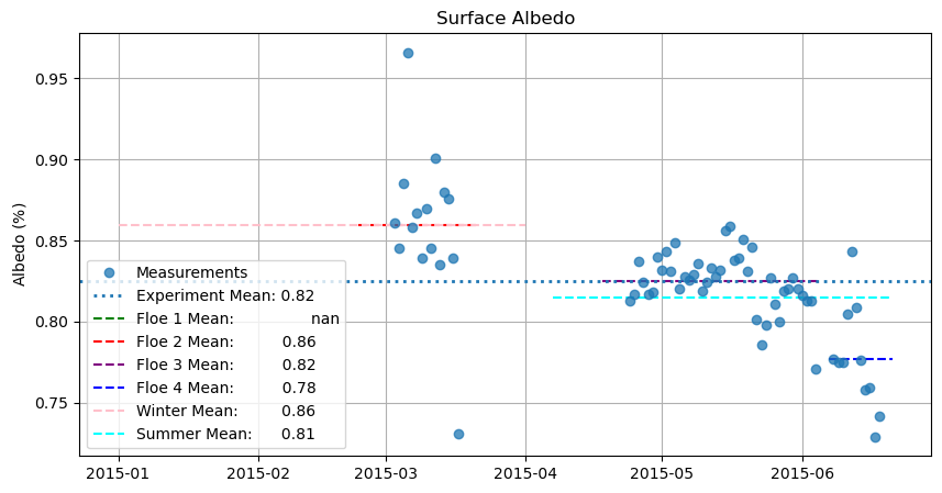
So we could increase the surface albedo to 0.86 in winter and 0.81 in summer